Bounded From Below — Four places a future disappears, and what to do first
I.
A forecast published this month puts global data center capital expenditure at $31.6 trillion through 2050. It runs five scenarios, publishes its methodology, and declines to weight any branch by probability. It is one of the better pieces of scenario work I have read in some time.
Every one of its five scenarios goes up.
The range runs from roughly $22 trillion to $50 trillion. The chip-constraint case halves annual spending by 2030 and recovers to finish above the central case by 2050. The sovereignty case moves the total by under seven percent and redistributes the rest. The slow-adoption case removes about $10 trillion and leaves buildings half empty, and the curve still rises. Across every branch, spending climbs.
That is a scenario floor: the level below which no branch in the set descends, whatever the set varies. A floor marks the boundary of what an exercise was built to be able to say, which is a different thing from a forecast of a minimum.
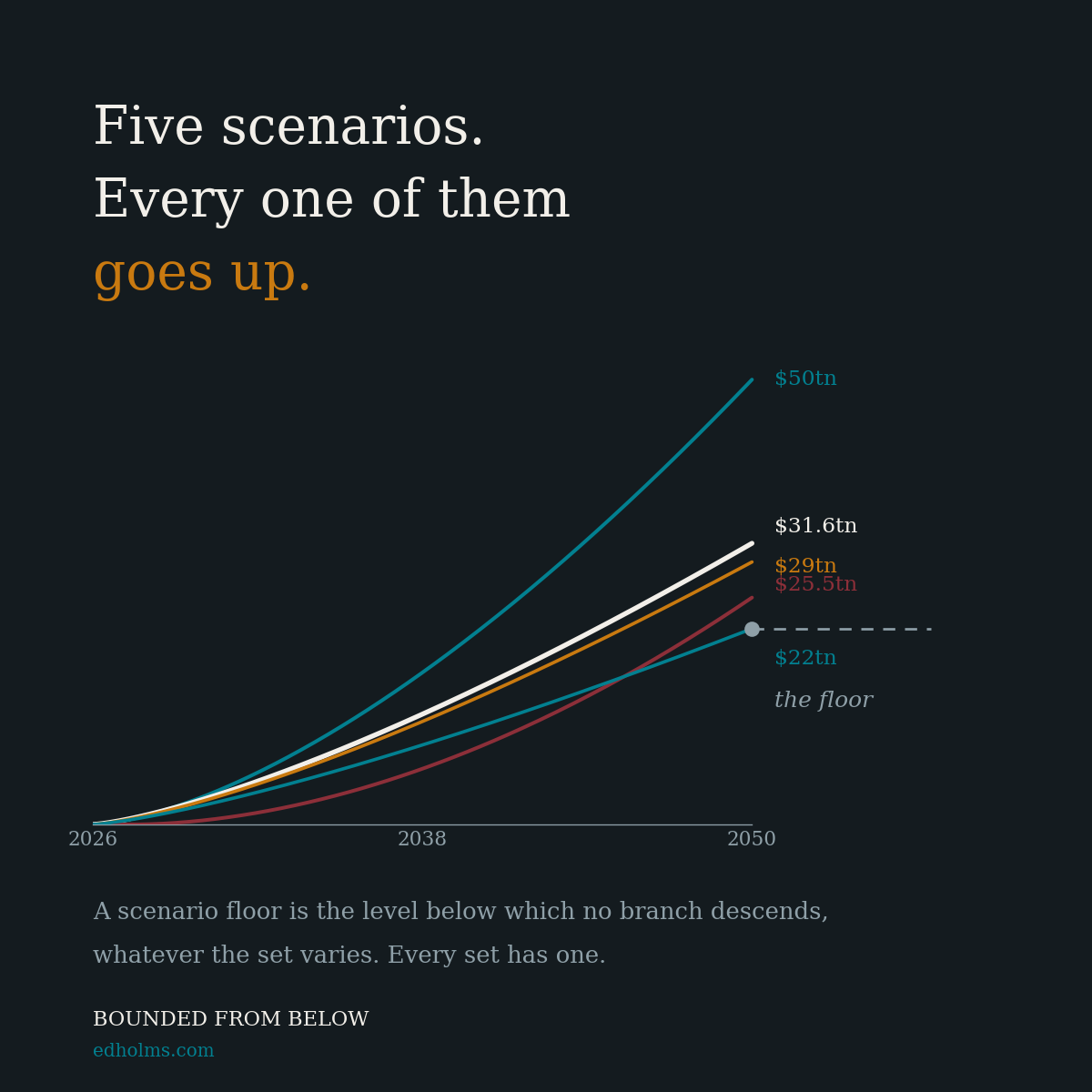
Every scenario set has one. The question worth asking of any set is not whether its range is wide enough, but what put the floor where it is.
II.
Where futures disappear
A scenario set is bounded by the architecture that produces it, and that architecture fails in four distinct places.
Measurement. The unit of account excludes the future entirely, so nothing downstream can recover it.
Model. The future is representable, but the variables and the relationships between them never generate it. It is thinkable and unthought.
Selection. The exercise generates the future and writes it down, and then someone removes it, softens it, or simply never carries it into a decision.
Phase. The constraints that bound the space run on different clocks, and the model holds them in step by construction. Timing mismatches do not appear as scenarios because the set varies magnitudes.
Each of the three documents below fails at a different point. None of them fails through carelessness, and one of them documents its own boundary in writing.
III.
Measurement: a trend line bent by the thing it measured
In April 2001, Mary Meeker and her colleagues at Morgan Stanley published an analysis of the technology downturn then underway. Its conclusion was that the correction would take two to six quarters to work through.
The document deserves better than its conclusion. It assembled forty years of business capital equipment spending split into IT and non-IT, twenty-one years of technology financing counted by category, manufacturers’ inventory against spending back to 1969, and quarterly revenue and earnings-surprise data across four hundred and fifty companies. Little of this existed in one place before.
The analysis built on it is careful. The authors separated excess spending attributable to over-financing from excess attributable to everything else, and reported the second as much larger. They noticed venture funding running at three times initial-offering proceeds against a decade median of one, and drew the correct inference that the venture business faced a worse reckoning than the public markets. They flagged an inventory divergence with only two precedents in thirty years.
The estimate was still wrong, for a reason worth more than the miss.
The trend line used to measure the excess had been fitted through the years the excess occurred. On that basis, overspending from 1998 to 2000 came to about $19 billion, roughly one percent of total IT spending. Three months after the report appeared, Nortel lost $19.4 billion in a single quarter, most of it writing down goodwill from acquisitions made during those same three years. One company, one quarter, matching the estimate for an entire industry over three. The bubble had raised the yardstick used to measure the bubble.
More data would not have caught this. The trend line was not a variable in the analysis. It was the instrument.
The report also concedes, in its own summary, that the largest single driver of the spending boom was business enthusiasm rather than the financing machinery the authors had just spent twenty pages quantifying. Greenspan had named the same thing in December 1996 and called it irrational exuberance; he was warning about it in advance, and the market ran for another three years regardless. Meeker reaches the same explanation from the far side, as a residual.
Enthusiasm is the name a quantitative model gives to the part of the world it cannot reach. If enthusiasm drove the spending, a trend line fitted to spending was tracking a symptom — which is precisely why it could not detect the excess running through it.
IV.
Model: the branch that cannot be generated
The 2050 forecast improves on that in specific ways. It publishes its methodology. It runs five scenarios rather than three. It declines to weight them by probability and says the alternatives describe coherent departures rather than ranked risks. And it names its own exclusion, stating that quantum computing sits outside the modeled range rather than inside it as a low-probability case.
That last point deserves emphasis. The 2001 report excluded its central assumption invisibly. This one identifies a discontinuity, decides to leave it out, and writes the decision where a reader can find it. Twenty-five years of real methodological progress sits in that difference.
The floor is still there, and the report is candid about what would break it. It observes that because capital expenditure must keep rising for decades, the revenue supporting it has to keep rising too, and that if adoption stalls or pricing weakens, the later years become harder to fund. That is the failure case, stated clearly, in prose. It never becomes a scenario.
The reason it cannot is visible in the methodology. The forecast is denominated in megawatts of IT load. The model works in megawatts and derives expenditure by applying construction and equipment cost benchmarks to that capacity. Performance improvements appear as more work per megawatt rather than as falling cost per megawatt, and no structural break in chip pricing is assumed in either direction.
Those are coherent choices, and they are the choices that make an architectural break unreachable. A technology that changes what a megawatt buys by an order of magnitude cannot enter a model in which the megawatt is the anchor.
So the exclusion of quantum owes nothing to discomfort. A measurement decision taken before any scenario existed had already put it out of reach.
V.
Horizon: how far to look, and what to count
Paul Saffo’s first rule of forecasting is to map a cone of uncertainty, and this report follows it — its own text describes the capital requirement as a cone widening with the horizon. His fifth rule is to look back twice as far as you look forward, in order to perceive the patterns underlying the change and find the constant hiding beneath the novelty. He adds a warning: forecasters too often use history for support rather than illumination.
The report does look back, and does it the way he warns against. It prices UK and US railway construction from 1840 to 1900 at about $0.72 trillion in today’s money, and the internet build-out from 1996 to 2001 at about $3.29 trillion, to establish that $31.6 trillion dwarfs both. That is history as a denominator — support for the scale of the claim rather than illumination of what the period contained.
Run for illumination instead, the arithmetic is unforgiving. Twenty-four years forward means forty-eight years back, to 1978. In 1978 the personal computer was a hobbyist product, and there was no public internet, no commercial cellular network in the United States, no fiber backbone, no graphics processor, no cloud, and no handset worth the name. A forecaster then, projecting data-processing capital expenditure to 2026, would have anchored on mainframe capacity and been wrong by category rather than by magnitude.
Forty-eight years of technological history does not establish which discontinuity will occur. It establishes that assuming none is a dangerous special case.
Saffo sends you back to find the constant. The same journey will tell you something he does not ask for, and events are the wrong unit for it — counting breakthroughs starts an argument about which ones qualify that never ends. Count redefinitions of the unit of account instead, and the answer is mechanical.
Look back twice as far, and count how many times the unit of account changed.
Depth alone does not supply that count, and the 2001 report proves it. Forty years of data behind a two-to-six-quarter forecast is a ratio of something like a hundred and sixty to one, far past what any rule requires. The look-back was deep and aimed at the wrong object: how much had been spent, when the question was how many times the thing being measured had been redefined.
Whether quantum computing transforms data centers is beside the point. What a scenario architecture needs is some way to represent something capable of doing so. The gap worth naming is the missing mechanism for discovering whatever eventually makes today’s unit of account inadequate.
VI.
Selection: the branch that does not travel
In 1995 the corporate strategy team at Ericsson built five futures for what telecommunications would look like in 2005, ten years out. Three were continuity scenarios, separated by which layer of the industry would drive its evolution: network, services, or devices. Two were discontinuity scenarios, one turning on a technological break and one on political upheaval.
Executive management approved all five for internal planning. Three left the building. The count is on the record, because the published account of the program names three.
The three that travelled went to industry forums, to a business school in France, to a graduate program in New York, and into executive sessions in Europe and Australia. The other two went into a drawer.
Four years later one of them happened.
That set failed Saffo’s fifth rule outright, and nobody in the room knew it: ten years forward, ten years back, half the distance the rule asks for. I learned the rule afterward, from Saffo and Bob Johansen at the Institute for the Future, in a conversation about the scenarios we had just finished.
Even at that shallow depth, the set generated both discontinuities. Measurement held. The model produced the branches. What failed came later.
The interesting part is which branch went missing. It was not, in my recollection, the least plausible one. It was the one whose truth would have made the rest of the planning pointless.
This is the failure point with the least excuse and the fewest defences. Measurement failures are invisible by construction. Model failures require someone to notice an absence. A selection failure happens in a room, to a document that already exists, in front of people who have read it.
VII.
Phase: constraints on different clocks
The fourth failure point has no obvious home in any of the three sets, and the 2050 forecast supplies all the parts.
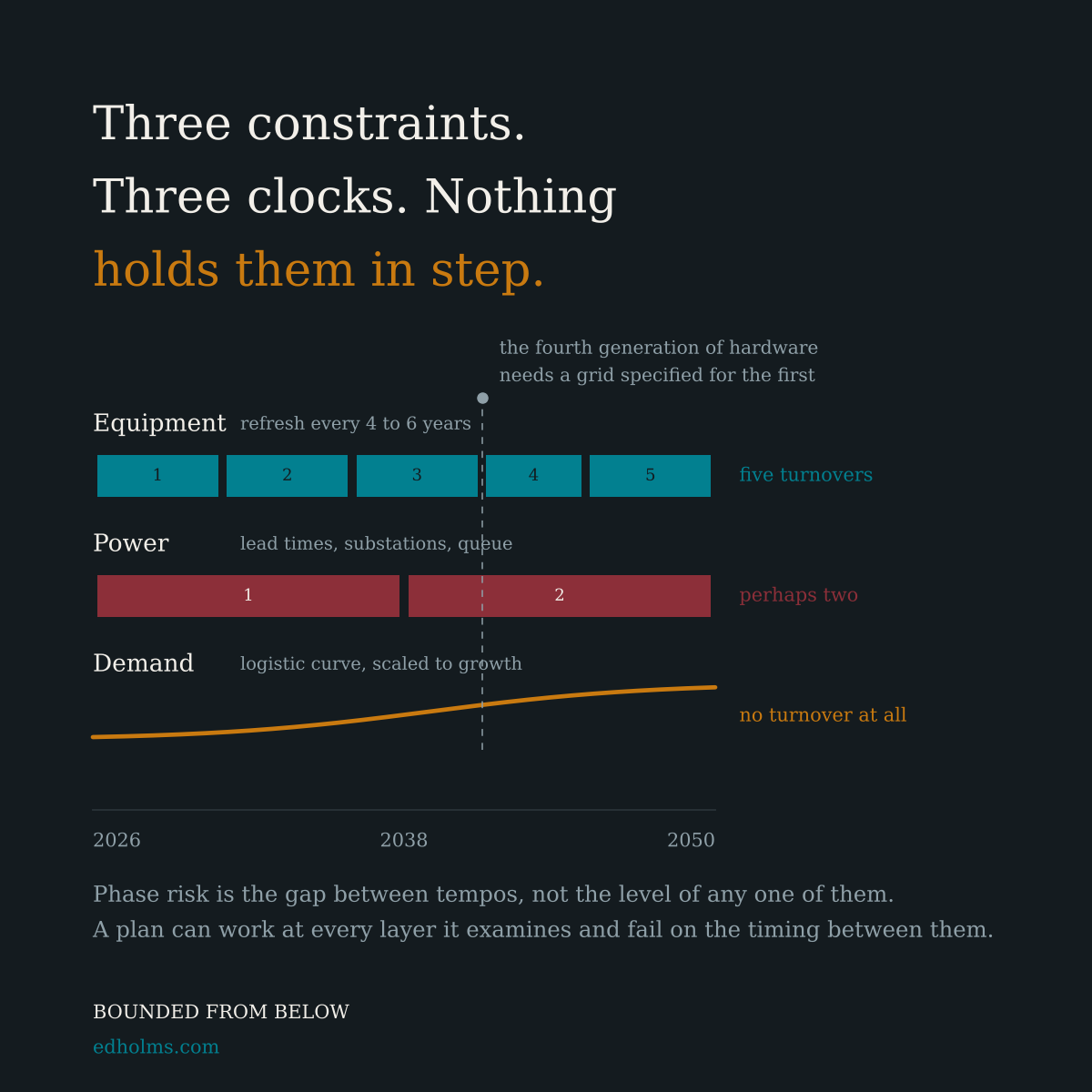
Silicon runs on a four-to-six year cycle. The document says so: three to five rounds of equipment investment inside a twenty-year asset life, with every dollar of construction committing roughly twelve dollars of future equipment spend, and equipment rising from seventy percent of total capital expenditure today to ninety-three percent by 2050.
Power runs on multiyear transformer lead times, substation availability, and transmission build. The report names it as the binding constraint under every scenario, including the ones where demand is lower.
Demand for applications and services runs on a logistic adoption curve scaled by economic growth. It is smooth by construction.
Three constraints, three tempos: one measured in years, one in decades, one continuous. Over twenty-four years each turns over a different number of times, and nothing in the model requires them to stay in step.
The mismatch the numbers imply is specific. The capital commitment sits overwhelmingly on the fastest clock. Whether any of it can be energized sits on the slowest. A grid specified for the 2030 generation of hardware must carry three or four later generations, none of which exist yet.
That is neither a demand risk nor a supply risk. It is a phase risk: the plan works at every level it examines and fails on the relative timing between them.
Why it hides
Phase risk is invisible to a set that varies magnitudes, because turning a variable up or down does not change when it arrives relative to anything else. Double the demand and the grid is still late. Halve it and the grid is still late, for fewer projects.
It also survives sensitivity analysis, which moves one input at a time and holds the rest at their central values. Phase risk lives in the relationship between two inputs, so testing each alone shows nothing. Both can sit comfortably inside their ranges while the gap between them opens.
And it hides behind aggregation. A twenty-four-year total conceals the sequence that produced it. Two paths to $31.6 trillion, one where capacity arrives when the hardware does and one where it arrives four years late every cycle, are the same number and different worlds.
The pattern is not confined to compute. Vaccine manufacture in 2020 ran into it — the industry solved doses before vials and cold chain, all three inside their own forecasts, none of them in step. Electric vehicles have a version now, with model programs on a four-year cycle and charging infrastructure on a permitting clock nobody controls. Wherever a plan depends on two constraints with different natural tempos, it is available.
What to do about it
The remedy is cheap and nobody runs it, which is the usual signature of a structural blind spot rather than a hard problem.
Start by writing down the tempo of every binding constraint, in the units the constraint actually moves in: refresh cycles, permitting timelines, hiring lead times, contract terms, depreciation schedules. Most plans have four or five, and most planning documents record none of them.
Then find every place the plan requires two of those clocks to stay in step, and mark it. The marks are the phase risks. They are usually few and usually obvious once written down, which is why the exercise takes an afternoon rather than a quarter.
For each one, ask what the world looks like when the faster clock has turned over twice more than the slower. That question generates a branch that no magnitude scenario contains, and it generates it without requiring anyone to forecast anything.
Then design against the gap rather than trying to close it. Phase risk is rarely fixable and frequently absorbable. Reserve grid capacity ahead of the hardware decision that will need it. Standardize the interface between the fast layer and the slow one so the fast layer can turn over without renegotiating the slow one. Take options on the slow constraint early, since options on slow things are cheap precisely because nobody wants them yet.
The last of those is the one worth pressing. An organization that has identified its phase risks knows which of its slow constraints to buy first, and slow constraints are the only ones still available to buy by the time everybody else notices.
VIII.
The boundary test
The remedy is a step taken before the model exists, and it has four parts, one for each place a future disappears.
Probe the unit of account. Name the unit the forecast is denominated in, then ask what would make it inadequate. Look back twice the horizon, as Saffo’s rule directs, and count the redefinitions rather than the events. A period that redefined its unit three times is telling you the probability of zero redefinitions ahead is not high. The output is a list of developments that would require a different unit, held open as a category rather than offered as a prediction of the next break.
Probe for the voiding future. Ask directly which single future would make the exercise pointless, and write it down. It carries no probability and needs none. The 2050 forecast already contains its own answer in prose: capital expenditure must rise for decades, so revenue must too. Moving that sentence into the model costs nothing and changes the shape of the set.
Probe the constraint structure. Name three things the system must deliver together, establish that any two can be had at the expense of the third, and read the scenarios off the corners. Energy policy has run on cheap, clean, and secure for decades — useful less for predicting prices than for foreclosing the branch in which all three improve, which is otherwise the branch everyone writes. Supply chains have their version in fast, cheap, and resilient, whose neglected corner arrived in 2020 with some force.
For a compute buildout the candidate is power: affordable, increasingly low-carbon, and delivered inside the interconnection lead times that determine when projects break ground. The forecast under discussion identifies all three and models them separately. Taken together as a trilemma, the third corner acquires content — a world where the constraint on the buildout sits outside the demand model entirely.
Probe the clocks. Inventory the tempo of every binding constraint, mark each place the plan needs two of them in step, and treat each mark as a branch. Set out at greater length above, and the cheapest of the four to run.
Then a fifth thing, which is not a probe. Assign each uncomfortable branch an owner before anyone writes it, and make finishing it that person’s job rather than the group’s. Selection failures happen to orphans.
None of these requires better data than the exercises above already had. Two of the four can be run against a document that is already finished.
IX.
What the remedy buys
None of this makes the $31.6 trillion figure wrong. The forecast may prove close. The three Ericsson scenarios that travelled described the destination well enough, and the two left in the drawer would not have changed the numbers anyone was given.
They would have changed what the company was ready for, and that is a different currency.
Accuracy is worth less than it looks. A central estimate that turns out correct tells an organization what happened, at the same moment everyone else finds out. A branch that was written, owned, and rehearsed tells it what to do on the morning the world moves, and it tells it before the room has finished arguing about whether the move is real.
The problem is rarely that organizations lack foresight. It is that the architecture connecting foresight to decisions has holes in it, and the foresight process has an architecture of its own that decides which futures are visible in the first place.
Finishing the uncomfortable branch does not improve the forecast. It shortens the reaction time when the branch nobody wanted turns out to be the one you are living in.
Sources and notes
Mike Edholm has spent three decades advising corporations and institutions on scenario planning and strategic foresight, with assignments spanning telecommunications, computing, industrial automation, and international development. This essay is part of a series on scenario planning methodology.